
Abstract
An EAF cooling system is classified as an auxiliary utility and functions as a life-preservation system. It is also the least legible part of the furnace: the operator is given a flow, two temperatures and two pressures per circuit, and must infer everything that matters from them.
Water-cooled panels, roof sectors, off-gas ducts, elbows and burner blocks allow modern Electric Arc Furnaces (EAFs) to operate at high power density while protecting metallic structures and surrounding equipment. Their condition cannot be understood reliably from outlet temperature, flow and pressure thresholds alone. Cooling performance is coupled to arc radiation, scrap shielding, foamy slag, burner and oxygen operation, furnace geometry, coolant distribution, scale formation and repeated thermal cycling.
Published EAF research has addressed radiative heat transfer, conjugate heat transfer within individual panels, cooling losses, first-principles furnace modelling and digital-twin-based optimisation. Separate advances in reduced-order modelling and hybrid physics–machine-learning systems show how high-fidelity physical models can be combined with plant data for rapid state estimation. These strands have not yet been integrated into a real-time reasoning architecture for EAF cooling.
This paper proposes a Physics-Grounded AI framework that reconstructs the unmeasured thermal and hydraulic state of an EAF cooling system from plant measurements, mechanistic models and high-fidelity simulation. The system represents spatial heat flux, panel-metal temperature, coolant state, thermal resistance, deposited scale, fatigue exposure and safety margin as one coherent physical state. It then reasons over that state to identify the mechanism behind abnormal behaviour, estimate future risk, and evaluate bounded operational responses — while declaring explicitly which circuits it cannot estimate and refusing to issue advice that rests on them. High-fidelity CFD and thermal analysis remain the verification layer rather than being replaced by AI.
The objective is to move EAF cooling from threshold-based monitoring towards physically explainable operational decision support.
1. Introduction
The cooling system of an Electric Arc Furnace is often classified as an auxiliary utility. Operationally, it is closer to a life-preservation system.
Water-cooled sidewall panels, roof sectors, off-gas ducts, elbows, burner blocks and related components remove heat that would otherwise damage metallic structures and shorten furnace campaign life. Research has shown that panel behaviour is shaped by both furnace-side radiative loading and coolant-side thermo-hydraulic response [1, 3]. Numerical studies identify local hot regions associated with stagnation, flow reversal and geometry near bends, while transient roof-panel studies connect repeated temperature variations with thermal fatigue and cracking [2, 4].
Most plant systems nevertheless expose the operator to measurements rather than physical state:
These measurements are essential. They do not reveal:
- local furnace-side heat flux;
- local tube or panel-metal temperature;
- flow maldistribution inside the panel;
- partial blockage or scale growth;
- local boiling margin;
- loss of protective slag coverage;
- cumulative thermal-fatigue exposure;
- remaining margin before damage.
The central proposition of this paper is:
An EAF cooling system should not be represented as a collection of water-circuit tags. It should be represented as an evolving thermo-hydraulic state constrained by furnace physics.
This is the role of Physics-Grounded AI [11].
2. Technical Background
2.1 Heat transfer to EAF cooling components
The inner surfaces of an EAF are exposed to intense and strongly non-uniform thermal loading. The principal mechanisms include radiation from the arcs, radiation and convection from molten steel and slag, chemical energy from burners and oxygen reactions, transient exposure following scrap movement, and changing shielding caused by foamy slag and scrap geometry.
A simplified local panel energy balance is:
where is incident radiation, is furnace-side convection, is heat transferred to the coolant, and represents transient energy storage in the panel material and deposits.
For an individual circuit, measured water-side heat extraction is approximated by:
This is an integral quantity. It cannot determine whether the extracted heat is distributed uniformly across the panel or concentrated in a small damaging hotspot.
2.2 Conjugate heat transfer
An EAF panel is a conjugate heat-transfer system involving:
- radiative and convective loading on the furnace side;
- conduction through slag deposits, refractory or panel material;
- conduction through the tube wall;
- forced convection within the cooling channel;
- transient heat storage in solid materials.
The local coolant-side heat transfer is:
where depends on local velocity, hydraulic diameter, fluid properties, roughness, geometry and flow regime.
A fall in measured bulk flow does not uniquely identify its cause. It may result from a valve condition, pump behaviour, leakage, blockage or measurement drift. Similarly, a rising outlet temperature may arise from increased furnace load, reduced cooling effectiveness, or both. This ambiguity is why tag-level diagnosis is inadequate — and it is the specific problem the reconstruction exists to solve.
2.3 Cooling loss versus protective cooling
Cooling panels protect the furnace but also remove useful thermal energy. The engineering objective is therefore not to maximise heat extraction [5, 6]. It is to minimise the combined penalty of energy loss, damage risk and downtime while satisfying safety and productivity constraints.
The objective, with all terms monetised on a common basis, is:
subject to:
The optimum is a constrained operating region, not a maximum-flow condition. The weights are a plant-specific commercial decision and must be set with the customer rather than assumed.
3. Why Conventional Monitoring Is Insufficient
A conventional cooling monitor evaluates rules such as:
These rules remain essential as independent safety interlocks. They have four limitations as a basis for understanding.
3.1 Spatial blindness
Two panels may show the same outlet-water temperature while one is heated uniformly and the other contains a highly concentrated hotspot. The integral measurement cannot separate them.
3.2 Cause–effect ambiguity
A rising outlet temperature may be caused by increased arc exposure, collapsed slag coverage, low coolant flow, scale formation, gas entrapment, partial blockage or changing inlet conditions. These require different — in some cases opposite — responses.
3.3 Reactive behaviour
By the time a bulk variable crosses a threshold, damaging thermal cycling or local overheating may already have occurred. Fatigue accumulated during the approach to the alarm is not recovered when the alarm clears.
3.4 Missing furnace context
Cooling load is affected by power-on state, arc length, burner activity, oxygen injection, scrap shielding, slag condition and process phase. A cooling alarm without process context may be technically correct and operationally incomplete.
4. From Data-Driven AI to Physics-Grounded AI
A conventional data-driven model estimates a future measurement [7]:
where contains measured cooling variables and contains furnace operating variables. Such a model can be accurate and still be unable to say why.
The Physics-Grounded formulation inserts a physical state between measurement and action:
where is the latent physical state and is a recommended operational or maintenance action. The state is:
Two consequences follow from making explicit. The estimate is tested against conservation laws, and the mechanism behind an abnormality is attributed rather than pattern-matched. Neither is available to a model that maps measurements directly to predictions.
5. System Architecture
5.1 Plant measurements
The required instrumentation is organised below under the four signal classes the GOATAI engine consumes. This application is carried principally by thermal and telemetry signals; imaging is optional and is not part of the minimum configuration.
| Signal class | Inputs for this application |
|---|---|
| Thermal | Circuit inlet and outlet water temperature; shell and panel-body temperatures where available; off-gas temperature |
| Telemetry | Circuit flow; inlet and outlet pressure; furnace electrical variables; burner and oxygen state; electrode position or arc-length proxy; process-phase markers; roof position; water-quality indicators |
| Geometry | Panel and header topology; circuit-to-position mapping; shell and bay geometry; as-built deviation where recorded |
| Imaging | Optical and acoustic indicators where feasible — foaming index, slag-coverage proxies. Not required for the minimum configuration |
Existing hardwired trips must remain independent. The system operates advisory-first: it warns, and the operator decides. It does not replace safety PLC logic and does not own the stop.
5.2 Mechanistic furnace model
A system-level model estimates energy generation and distribution through electrical input, chemical energy, scrap and bath heating, reaction enthalpies, off-gas losses, wall and roof losses, and cooling-water heat extraction [6, 8].
The model provides physically plausible global energy allocation even where local measurements are sparse, and supplies the incident-energy term against which the reconstruction is closed.
5.3 High-fidelity local models
Detailed CFD and conjugate thermal models are developed for representative sidewall panels, roof sectors, delta regions, burner blocks, off-gas elbows, ducts, bends and headers [1, 2, 3].
These models identify recirculation zones, reverse flow, stagnation, local wall-temperature maxima, transient gradients, boiling margin and geometry-specific pressure loss. They are the source of the reduced representation and remain the verification layer throughout deployment.
5.4 Reduced physical representation
High-fidelity fields are too expensive to solve continuously. They are compressed using reduced-order representations [9, 10]. For a temperature field:
where are spatial basis modes and are reduced coordinates.
Separate reduced bases are required for physically distinct regimes: high arc exposure, shielded scrap, stable foamy slag, slag collapse, burner-dominant heating, charging, and roof-open transients. A state that falls between bases, or outside all of them, is an abstention condition and is treated as such.
5.5 State estimator and instance grounding
Plant measurements update the reduced physical state through an Ensemble Kalman Filter, Unscented Kalman Filter, Moving Horizon Estimator, Bayesian filter, or a learned observer constrained by physical residuals:
Slowly varying parameters within — surface roughness, effective thermal resistance, scale thickness, effective flow area — are estimated jointly with the fast state and carried as degradation indicators.
This joint estimation is the mechanism of instance grounding. A generic panel model describes a class of panels. Continuous reconciliation of against one installation's measurements produces a model of this furnace, on this campaign day, with the scale and wear it actually has — and keeps that model current as the installation ages and drifts. The distinction is not incidental to the method; it is the method. A model that does not track will attribute the slow drift of a degrading circuit to fast process variation, and will do so with increasing confidence as the campaign progresses.
5.6 Physics residuals
The inferred state is continuously tested against conservation laws.
Energy residual:
Mass residual:
Hydraulic residual:
Persistent residuals indicate blockage, scale deposition, leakage, gas entrainment, sensor bias or unmodelled furnace events.
Residuals serve two distinct functions and the distinction matters. As diagnostics, a residual localises a fault. As an admissibility gate, a residual outside its band disqualifies the reconstruction as a basis for advice, irrespective of the confidence the estimator reports internally. The second function is the stronger one.
6. Physics-Grounded Reasoning Modes
The four modes below correspond to the four stages of the GOATAI reasoning engine. Each consumes the state rather than the raw measurements.
6.1 Monitoring — present-state estimation
The system estimates present spatial heat flux, peak metal temperature, hydraulic state, thermal safety margin, and the uncertainty attaching to each. Uncertainty is reported per quantity. A directly instrumented flow margin and a long-horizon remaining-life extrapolation do not share a confidence value, and must not be presented as though they do.
6.2 Prediction — short-horizon state
Predictions report calibrated uncertainty and abstain when the state lies outside the validated domain of the reduced representation.
6.3 Reasoning — mechanism attribution
The system distinguishes furnace-side loading from coolant-side degradation. It concludes that the outlet-temperature rise is driven by increased radiation following slag collapse rather than by a reduced heat-transfer coefficient.
Attribution is performed on the series-resistance decomposition. Because , the temperature rise from coolant bulk to hot face decomposes to scale across the chain — coolant film, internal deposit, tube wall — and the segment that has grown identifies the mechanism directly. Two circuits at the same metal temperature with different segment distributions are different events requiring different responses.
Where two mechanisms remain consistent with the available evidence, the system reports both with their posterior weights and identifies the measurement that would discriminate between them, together with its cost. It does not select the more likely mechanism and present it as the finding.
6.4 Decision — bounded counterfactual evaluation
Candidate actions may include increasing circuit flow within hydraulic limits, altering burner or oxygen sequence, restoring foamy slag, changing electrical operation, redistributing arc exposure, shortening exposure, scheduling inspection, or reducing power under defined safety conditions.
The decision objective:
Two disciplines apply. First, the recommendation balances safety, energy efficiency, production and asset life rather than minimising temperature. Second, the action set must be partitioned at the outset into variables the operator can move during the present heat and variables fixed for the campaign — shell configuration, panel construction, header topology, pump capacity. Where the binding constraint lies inside the fixed set, the correct output is a statement to that effect, not an optimisation over the variables that remain. A system that optimises a reachable variable while the binding one is out of scope produces a confident recommendation that cannot work.
7. Abstention and Observability
Not every circuit can be estimated, and the system's value depends as much on saying so as on the estimates it does produce.
7.1 Three observability classes
Every circuit is assigned to one of three classes, and the class is reported alongside every estimate:
- Direct — individually instrumented. Inlet and outlet temperature, flow and pressure available at circuit level.
- Inferred — reconstructed from header-level measurements and the mechanistic model. Estimated with a materially wider uncertainty band, and labelled as such.
- Abstained — insufficient evidence to support any estimate. Reported as unestimated. No value is imputed.
A shell instrumented at header level with selective circuit-level instrumentation will contain all three classes simultaneously. Presenting the third as nominal — because a blank cell is visually awkward, or because a downstream consumer expects a complete vector — converts an honest gap into a false reading.
7.2 Abstention conditions
The system abstains from issuing advice when any of the following holds:
- the reconstruction lies outside the validated domain of the reduced representation;
- a conservation residual falls outside its admissible band, rendering the reconstruction inadmissible regardless of internal estimator confidence;
- the advisory would rest on one or more circuits in the abstained class;
- two or more mechanisms remain consistent with the evidence and the proposed action does not discriminate between them.
An action that relieves a symptom under either of two competing mechanisms appears attractive: it works whichever is true. It is nonetheless the wrong recommendation, because it consumes margin, leaves the actual cause in place, and destroys the observation that would have discriminated. The correct output is the discriminating measurement.
7.3 Reporting
Abstention is reported as a first-class output, not as a gap in a display. Every advisory carries the observability composition of the circuits it depends on, the residual state at the time of issue, and confidence stated per claim rather than as a single scalar over the whole inference.
This is the operational meaning of the requirement that a physics-grounded system know the limits of its own knowledge [11].
8. Presenting the Reconstructed State
A reconstructed state is useful only if it can be read correctly under operating conditions — on a pulpit display, at distance, by an operator managing a heat. This section states the presentation requirements, shows a widely proposed format that fails them, and gives the alternative.
8.1 Four requirements
R1 — Single-valued directionality. Every axis of a summary must point the same way. Mixing "higher is better" margins with "lower is better" risk indices on one figure makes the geometry unreadable whatever the axis labels say.
R2 — Load and degradation on separate channels. An elevated panel-metal temperature has two independent causes: increased net absorbed flux, or increased thermal resistance. A single colour scale or a single score fuses them. They require different responses.
R3 — Abstention visible. Circuits in the abstained class must be shown as unestimated, and must be visually distinguishable from circuits estimated at a low value.
R4 — Margin, not score. The operator requires distance to a limit in physical units and the time available before it is reached. A normalised health index supplies neither.
8.2 Why a radar summary fails all four
Figure 1 shows a cooling health overview of a kind frequently proposed for this application.
It violates R1. Four of the ten axes are risk indices for which lower is better; six are margins for which higher is better. All ten are plotted against a convention in which the outer edge is good and the inner alert ring is unacceptable. The consequence is visible in the figure itself: leakage risk index 18 — a good value — plots deep inside the alert ring, while the accompanying interpretation panel correctly describes leakage risk as low. The geometry and the text state opposite things. On a control-room display, where shape is read at distance and numbers are not, the geometry wins.
It violates R2. Heat flux margin, panel metal temperature margin, scaling index and hotspot severity all resolve to position on a common radial scale. A panel running hot because its slag coverage has gone and a panel running hot because its tube is scaling produce similar polygons and demand opposite interventions.
It violates R3. All ten axes carry a value. There is no representation for a quantity the system cannot estimate, and no visual state between "estimated at a low value" and "not estimated".
It violates R4. A single model confidence of 0.87 is reported for a ten-dimensional inference spanning a nearly directly measured coolant flow margin and a long-horizon remaining-life extrapolation whose credible interval is far wider. Collapsing both into one figure is precisely the behaviour abstention exists to prevent.
Two structural defects compound these. Polygon area — the quantity the eye computes first — depends on the arbitrary ordering of axes around the circle and therefore carries no meaning. And composite quantities such as overall cooling effectiveness and remaining life estimate are plotted alongside the quantities from which they are derived, double-counting them and inflating the apparent dimensionality of the display.
The uniform alert ring is a third. A limit set at an identical normalised value across heat flux, pressure drop, deposit fraction and remaining life was not derived per quantity. Any furnace engineer reading the figure will identify this immediately, and it undermines the claim of physical grounding that the same figure asserts.
Counter-example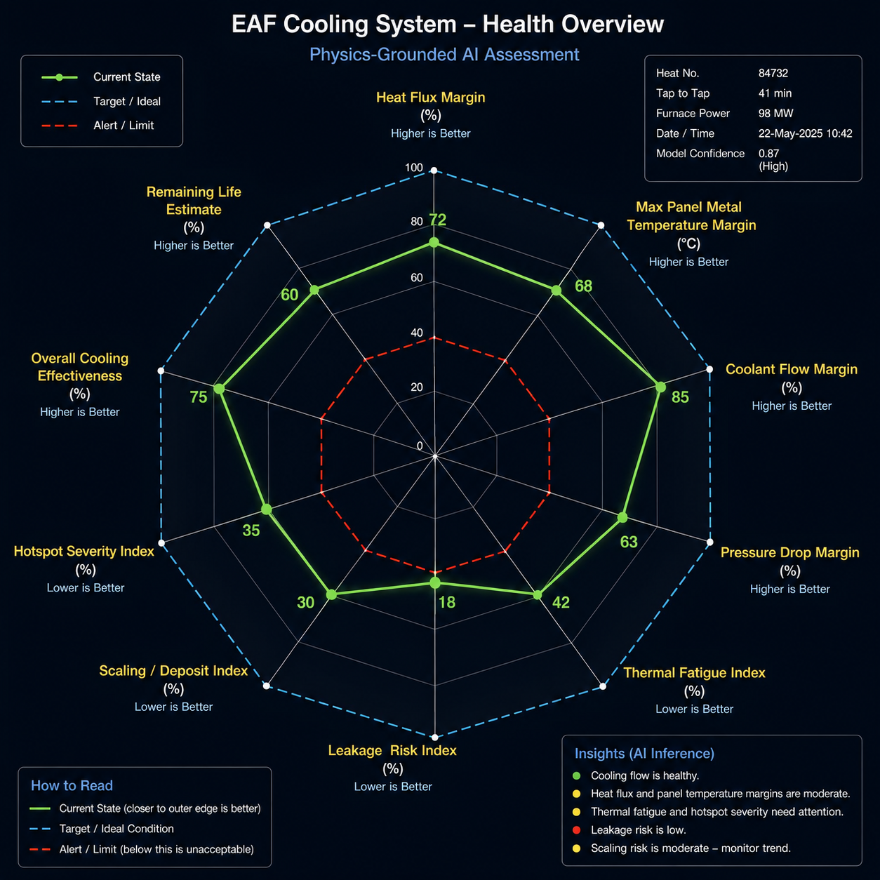 Figure 1. A cooling health overview of the kind this paper argues against. Retained as a worked counter-example. Values are illustrative.
8.3 Field-native presentation
The alternative uses the plant's own geometry as the display substrate and separates the two causal channels.
Developed shell map (Figure 2). The furnace shell is unrolled into a rectangle: circumferential angle 0–360° on the horizontal axis anchored to real landmarks (taphole, slag door, electrode phases, burner positions), elevation on the vertical. Each cell is a physical cooling circuit at its true position, with the off-gas elbow and duct carried as a separate strip.
Adjacency performs the diagnosis without further encoding. A hot band spanning several neighbouring circuits at one azimuth is coverage loss. A single hot circuit between healthy neighbours is a circuit-side problem. Both are legible on a spatial map. Neither survives dimension reduction.
Within each cell, load and degradation occupy separate visual channels, satisfying R2:
- fill colour encodes net absorbed heat flux — the load;
- hatch encodes excess thermal resistance — the degradation, on a visual channel deliberately opposed to the heat scale;
- a foot bar encodes coolant-side margin — distance to departure from nucleate boiling.
Circuits in the abstained class are rendered blank and outlined, satisfying R3.
The idiom has precedent in adjacent domains — blast-furnace stave flux maps, mould thermal maps for breakout detection, boiler waterwall fouling maps — and therefore requires no training to read.
Method demonstration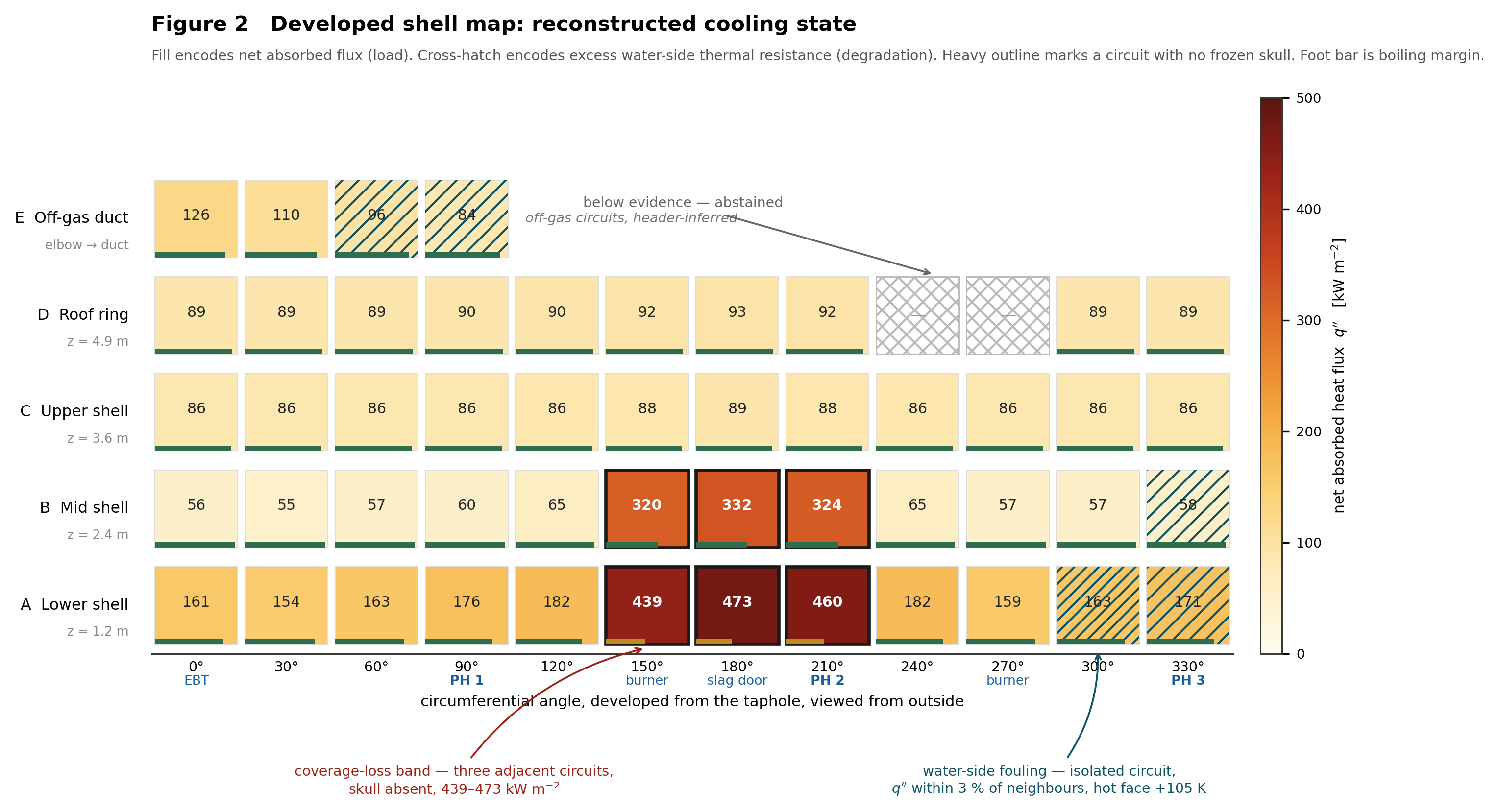 Open figure full size ↗
Figure 2. Developed shell map, unrolled 0–360°, viewed from outside. Fill encodes net absorbed flux; hatch encodes excess water-side thermal resistance; heavy outline marks a circuit with no frozen skull; foot bar encodes boiling margin. Cross-hatched white cells are abstained. Computed; see Appendix A.
Open figure full size ↗
Figure 2. Developed shell map, unrolled 0–360°, viewed from outside. Fill encodes net absorbed flux; hatch encodes excess water-side thermal resistance; heavy outline marks a circuit with no frozen skull; foot bar encodes boiling margin. Cross-hatched white cells are abstained. Computed; see Appendix A.
ΔT budget ladder (Figure 3). For any selected circuit, a stacked bar decomposes the temperature rise from coolant bulk to hot face across the series resistance chain: coolant film, internal deposit, tube wall. Because , the stack is the mechanistic model drawn to scale.
The figure resolves the case that defeats every scalar summary. A circuit at elevated flux with an unchanged resistance chain and a circuit at below-nominal flux with a large deposit segment reach comparable metal temperatures. Their stacks are unmistakably different, and their required responses are unrelated.
Method demonstration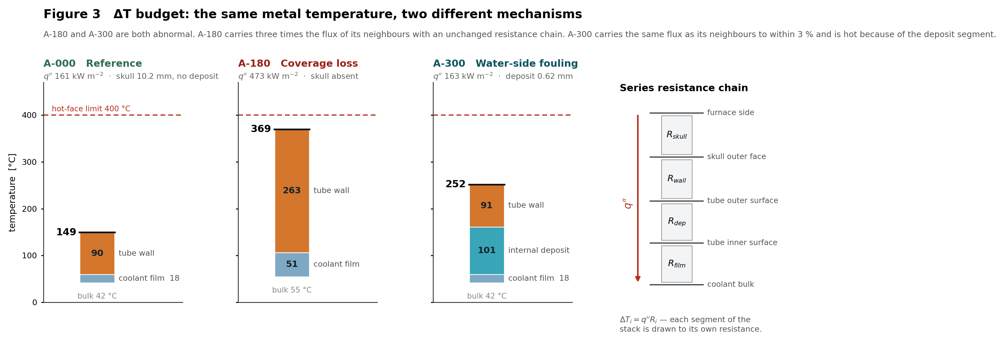 Open figure full size ↗
Figure 3. ΔT budget for three circuits — reference, coverage loss, and water-side fouling — with the series resistance network. Computed; see Appendix A.
Open figure full size ↗
Figure 3. ΔT budget for three circuits — reference, coverage loss, and water-side fouling — with the series resistance network. Computed; see Appendix A.
Closure and observability (Figure 4). Two elements complete the display. A closure bar compares measured total extraction against the integral of the reconstructed flux field, plotted against the full admissible band. Axes are fixed to the requirement and never autoscaled to the residual — an autoscaled residual axis renders a converged solution as visually unstable. Alongside it, an observability strip reports the composition of the shell across the three observability classes.
Method demonstration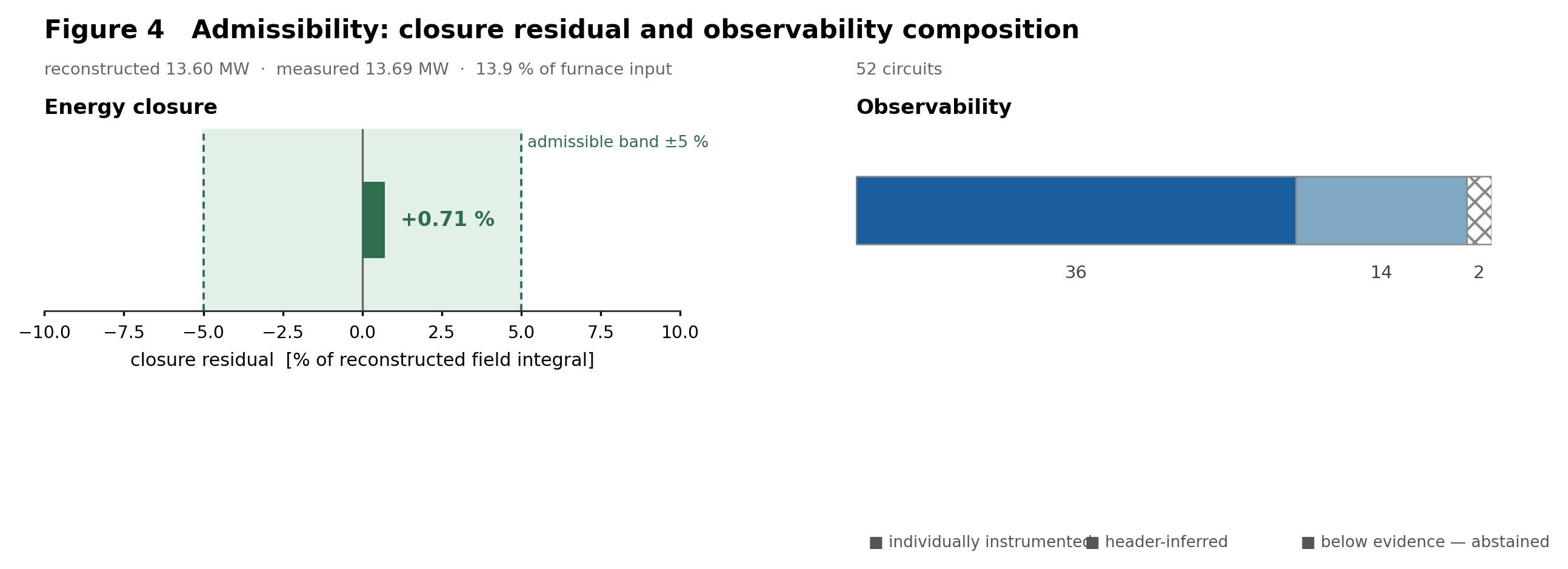 Open figure full size ↗
Figure 4. Energy closure against the admissible band, and observability composition. Computed; see Appendix A.
Open figure full size ↗
Figure 4. Energy closure against the admissible band, and observability composition. Computed; see Appendix A.
8.3.1 Computed behaviour of the three signatures
The figures are generated from the reduced model of Appendix A for a 98 MW furnace with a partial slag-door coverage collapse and a single fouled lower-shell circuit.
The two mechanisms are not separable on flux alone. Circuit A-300 carries 163 kW m⁻², and its unaffected neighbour A-270 carries 159 kW m⁻² — a difference of 2.5 %, inside the reconstruction uncertainty. Their hot-face temperatures differ by 105 K (252 °C against 147 °C). The load channel is silent; the entire signal is in the resistance channel. A display that fuses the two, or a scalar health index built from either alone, cannot represent this circuit.
The skull self-regulates, which is why fouling hides. Because the frozen slag layer thins until its outer face reaches the slag solidus, a circuit with added water-side resistance sheds skull thickness (9.2 mm against 10.2 mm at A-270) and absorbs almost the same flux. Water-side fouling therefore produces very little change in the measurable heat extraction while raising metal temperature substantially. This is an emergent result of the model, not an assumption placed in it, and it explains why fouling is routinely detected late.
Coverage loss is a cliff rather than a gradient (Figure 5). A skulled surface sits at the slag solidus and re-radiates 259 kW m⁻²; it absorbs only the excess above that floor. A bare panel sits a few hundred degrees above the coolant and re-radiates almost nothing. At the same incident irradiation the two states differ by a factor of 2.9 in absorbed flux. There is no gradual regime between them, which is why threshold monitoring on a slowly rising outlet temperature gives so little warning.
Method demonstration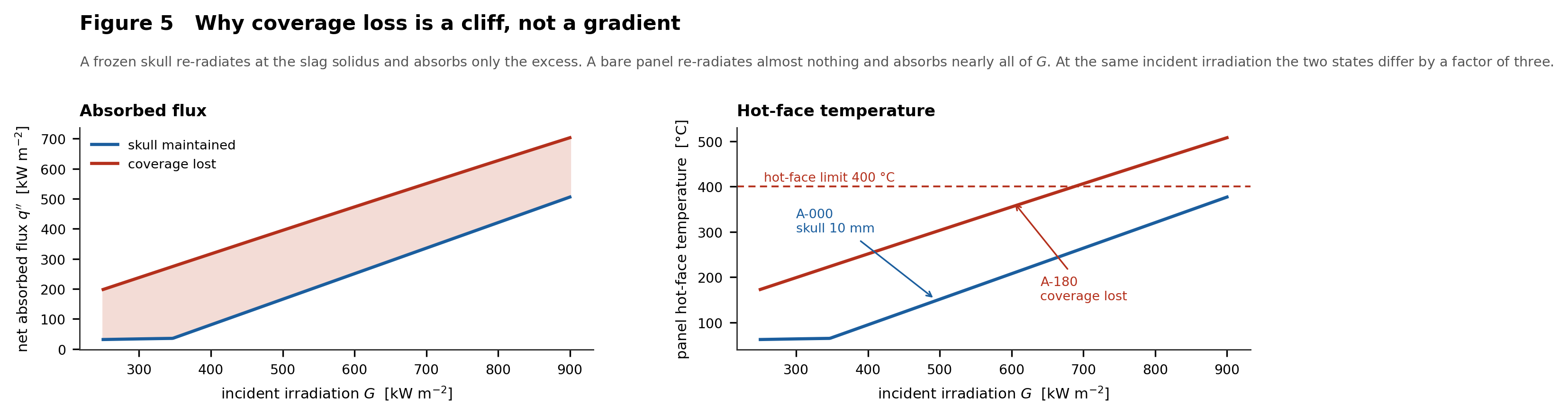 Open figure full size ↗
Figure 5. Absorbed flux and hot-face temperature against incident irradiation, for a skulled and a bare surface. Computed; see Appendix A.
Open figure full size ↗
Figure 5. Absorbed flux and hot-face temperature against incident irradiation, for a skulled and a bare surface. Computed; see Appendix A.
8.3.2 The energy consequence
Running the same model across three coverage states quantifies what the display is for (Figure 6):
| Scenario | Cooling load | Fraction of furnace input | Excess over full coverage |
|---|---|---|---|
| Full coverage | 9.68 MW | 9.9 % | — |
| Local collapse at the slag door | 13.60 MW | 13.9 % | 3.92 MW |
| Bath-wide foaming collapse | 25.35 MW | 25.9 % | 15.67 MW |
Both abnormal states raise outlet temperature on the circuits they affect. They differ by a factor of four in energy penalty and require different responses — local slag practice at the door in the first case, bulk carbon injection and arc regime in the second. A circuit-level threshold sees the same alarm in both.
Method demonstration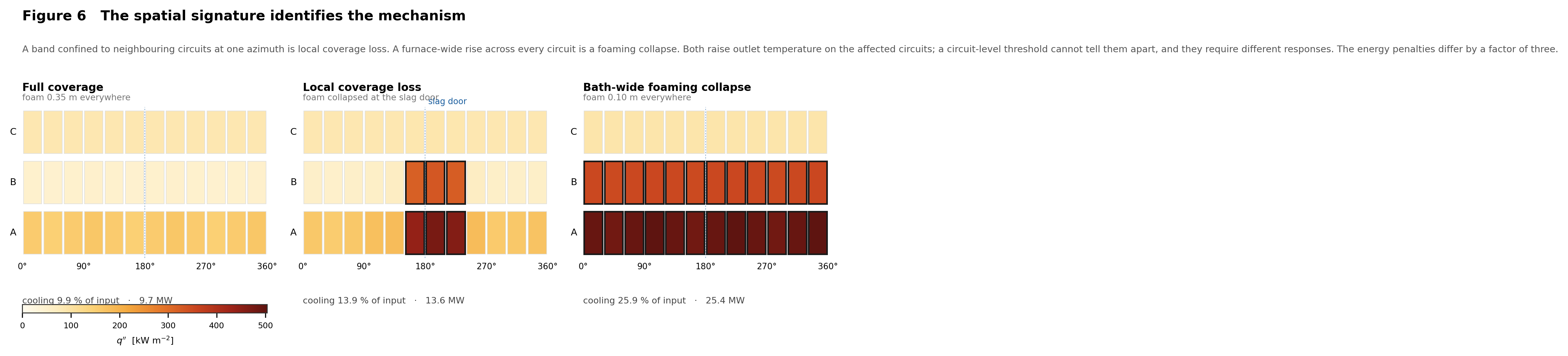 Open figure full size ↗
Figure 6. Reconstructed flux across three coverage states. Computed; see Appendix A.
Open figure full size ↗
Figure 6. Reconstructed flux across three coverage states. Computed; see Appendix A.
8.4 Two timescales
Cooling state contains fast and slow variables, and they do not share a display resolution. Heat flux, flow, pressure drop and metal temperature evolve within a heat. Scale growth, fatigue accumulation and life consumption evolve over days to weeks.
Presenting slow variables at heat resolution implies a sensitivity the physics cannot support and invites operators to attribute heat-to-heat noise to real degradation. Slow variables are carried on a separate trajectory panel, timestamped with their actual update interval, and expressed where possible as heats remaining to an intervention threshold rather than as a present value.
9. Illustrative Diagnostic Cases
9.1 Rising outlet temperature with normal flow
Measurements: outlet temperature rising; flow and pressure drop stable; arc current and burner input increasing; slag indicator deteriorating.
Reconstruction: incident heat flux elevated; resistance chain unchanged; inferred skull thickness reduced.
Interpretation: increased incident load with reduced shielding. No evidence of hydraulic degradation.
9.2 Falling heat removal with increasing pressure drop
Measurements: flow declining; pressure drop increasing; inlet conditions and furnace pattern stable.
Reconstruction: effective flow area reduced; hydraulic residual persistently positive.
Interpretation: increased hydraulic resistance consistent with scale growth or obstruction.
9.3 Normal bulk measurements with abnormal reconstructed local state
Measurements: normal circuit temperature rise; normal total flow; oscillatory pressure signature.
Reconstruction: local peak metal temperature substantially above the circuit-average value implied by the bulk measurements; boiling margin locally reduced.
Interpretation: internal maldistribution, local vapour formation, bend recirculation or partial blockage.
The hotspot is not measured — no instrument observes it. It is reconstructed, and it is invisible to every bulk quantity available at the circuit boundary. The oscillatory pressure signature is the only direct evidence, and by itself it is not diagnostic.
9.4 Repeated charging-cycle thermal shocks
A physics-grounded system accumulates a damage proxy rather than resetting when an alarm clears:
The objective becomes campaign-life management rather than present-temperature control alone. is a slow variable and is reported on the trajectory panel, expressed as heats remaining at the current accumulation rate.
10. Training and Validation Strategy
10.1 Offline physical model generation
Generate a simulation design space spanning heat-flux distributions, inlet temperatures, flow rates, pressure conditions, scale thicknesses, roughness, partial blockage, geometry variants and transient furnace events.
Each case retains geometry, boundary conditions, field solutions, convergence records, derived engineering quantities, uncertainty, and — critically — its validity range. The validity range is what makes the abstention condition computable rather than nominal.
10.2 Historical plant calibration
Historical heat data calibrates effective heat-flux distribution, thermal resistance, hydraulic resistance, sensor bias and phase-specific operating regimes. This is the initial instance-grounding pass; the continuous pass runs thereafter.
10.3 Controlled plant trials
Validation progresses through three phases: shadow mode (reconstruction runs and is recorded, no output to the operator), advisory mode (output presented, operator decides), and guarded optimisation (bounded actions within pre-agreed envelopes). Independent safety trips remain in force throughout all three.
10.4 Validation metrics
Evaluation includes outlet-temperature error, heat-extraction error, pressure-drop error, hotspot-location accuracy, peak-metal-temperature error, early-warning time, false-alarm rate, missed-event rate, uncertainty calibration, conservation residuals, and improvement in panel life or inspection accuracy.
Several of these metrics — conservation residual behaviour, uncertainty calibration, abstention rate against verified out-of-domain cases — constitute a measure of how well grounded a given deployment is. That measure is developed separately as a domain-independent construct; this application serves as its worked example.
11. Distinction from a Conventional Digital Twin
A conventional digital twin may mirror process variables or perform energy-balance simulation. The system adds four capabilities:
- reconstruction of unmeasured spatial thermal and hydraulic fields;
- mechanistic explanation of the observed state;
- counterfactual evaluation of bounded operational actions, verified against high-fidelity models;
- explicit declaration of what it cannot estimate, and refusal to advise on that basis.
The deployment pipeline is:
The deployment pipeline describes how information moves through an installation. The reasoning cycle of §6 describes what the system does with a state once it holds one.
12. Research Questions
- Can sparse circuit-level measurements reconstruct local panel heat-flux and metal-temperature fields with useful accuracy?
- Can a reduced-order model distinguish increased furnace heat load from degraded coolant-side heat transfer?
- Can slowly varying parameters such as effective thermal resistance, flow area and roughness indicate scale, obstruction and panel deterioration ahead of threshold crossing?
- Does arc, slag, burner and furnace-phase context reduce false cooling alarms compared with tag-only models?
- Can cumulative transient thermal-state estimates predict maintenance need earlier than conventional alarms?
- Can physics-based counterfactual analysis reduce cooling losses without increasing panel risk?
- Does explicit abstention on low-observability circuits improve operator trust and acted-upon rate relative to a system that always answers?
13. The Pilot
The pilot below is framed as the third stage of a co-creation engagement: technical deep-dive, site assessment, then staged joint proof-of-concept with success criteria agreed in advance and signed off as a business case.
Scope. One high-risk sidewall panel or one roof-cooling circuit.
Initial inputs. Inlet and outlet temperature, flow, inlet and outlet pressure, furnace power, oxygen and burner state, process phase, arc proxy, and any available local temperature measurement.
Offline model. A validated transient conjugate heat-transfer model of the selected circuit, with its validity range recorded.
Online outputs. Estimated incident heat load; peak metal temperature; inferred coolant-side condition; thermal margin; hydraulic anomaly score; short-horizon prediction; the dominant mechanism with its attribution; and the observability class of every quantity reported.
Phasing. Shadow, advisory, then guarded optimisation.
Success criteria. Earlier detection than existing alarms; correct discrimination between process-induced heating and cooling-side degradation; calibrated uncertainty; appropriate abstention on out-of-domain states; and engineering explanations accepted by furnace and maintenance specialists.
The weights are set during the first stage, with the customer. They encode a commercial judgement about the relative cost of energy, damage and downtime at that plant, and they are not a modelling choice.
14. Safety and Deployment Boundaries
EAF cooling is safety critical. Therefore:
- AI must not replace independent hardwired protection;
- prediction uncertainty must always be visible, and stated per quantity;
- recommendations must remain within approved operating envelopes;
- out-of-distribution states must trigger abstention;
- every advisory must preserve traceability to measurements, model state and evidence class;
- high-risk actions require operator confirmation;
- model changes require version control and revalidation.
The system is advisory-first by design. It warns; the operator decides. It does not own the stop.
15. Discussion
The technical literature provides much of the foundation this system requires: radiative heat-transfer models, transient conjugate heat-transfer models, energy-balance and first-principles EAF models, data-driven temperature prediction, digital twins, and reduced-order physical representations.
The remaining challenge is to integrate them around the operational object that matters — the evolving physical state of the cooling system — and to be disciplined about what that state cannot support.
A purely data-driven alarm model detects familiar patterns. A high-fidelity CFD model explains a specified scenario. Neither is sufficient alone for continuous plant reasoning. The practical architecture is hybrid:
To which one further term must be added, because it is the term that makes the rest usable on a furnace: a declared boundary of competence.
16. Conclusion
Electric Arc Furnace cooling is a coupled thermo-hydraulic and furnace-process problem, not a water-distribution problem.
Existing monitoring provides essential measurements but rarely reconstructs the physical conditions responsible for panel damage, excess energy loss or approaching failure. Physics-Grounded AI supplies the connecting architecture: it converts measurements into a coherent thermal and hydraulic state, tests that state against conservation laws, explains abnormal behaviour, predicts near-term risk, and evaluates alternative operational responses — declaring, throughout, which circuits it cannot see.
CFD and first-principles modelling remain central. They become the source of representation and the layer of verification rather than isolated engineering studies.
The result is not a cooling dashboard. It is a means for the person on the pulpit to know what is happening inside a panel they cannot open, during a heat they cannot pause — and to know when the system cannot tell them.
Appendix A — Reduced physical model
The figures are computed from a reduced model of the shell cooling system. It is not a substitute for the high-fidelity conjugate heat-transfer models, and it is not a validated plant model. Its purpose is to demonstrate that the presentation and reasoning arguments hold on a physically self-consistent field rather than on chosen numbers.
A.1 Formulation
Incident irradiation. Each cooling circuit is sub-discretised (30 elements per shell panel, 18 per roof sector). Incident irradiation on each element is the sum of three terms: three arc columns treated as isotropic line sources carrying the radiated fraction of furnace power; the melt surface treated as diffuse patches exchanging by the differential area-to-area relation; and a freeboard gas term. Arc contributions are attenuated through foam by a Beer–Lambert factor over the local foam depth. The melt surface radiates at a temperature interpolating between a covered foam top and exposed slag as local coverage fails. A single-bounce cavity factor accounts for inter-surface reflection, which is not otherwise resolved.
Fire-side surface state. Where molten slag is delivered — within the splash zone and above a minimum coverage depth — a frozen skull is assumed with its outer face at the slag solidus. Skull thickness follows from requiring the skull to conduct the net absorbed flux from the solidus to the panel surface. Where the required thickness is non-positive, no skull can be sustained and the surface is solved bare from its own radiative balance. Outside the splash zone a dust and oxide crust is carried in place of a skull.
Series chain and coolant side. Behind the fire-side surface the chain is tube wall, water-side deposit and coolant film. The film coefficient follows Dittus–Boelter and is referred to the panel face area through a wetted-area ratio. Circuit bulk temperature is iterated with the absorbed heat.
Closure. The reconstructed field integral and the measured circuit extraction are computed independently. The measured side is simulated by applying flowmeter bias and RTD noise at the magnitudes declared below, so that the closure residual in Figure 4 is an instrument-limited discrepancy rather than an identity.
A.2 Parameters
| Group | Parameter | Value |
|---|---|---|
| Geometry | shell inner radius | 3.20 m |
| melt surface radius | 3.00 m | |
| electrode pitch-circle radius | 1.10 m | |
| panel rows above sill | 1.20 / 2.40 / 3.60 m | |
| roof ring elevation | 4.90 m | |
| sectors per row | 12 | |
| Sources | furnace electrical input | 98.0 MW |
| radiated fraction from arc columns | 0.28 | |
| arc length | 0.45 m | |
| covered (foamed) surface temperature | 1748 K | |
| exposed slag / steel temperature | 2123 K | |
| freeboard gas emissivity, temperature | 0.15, 1873 K | |
| cavity augmentation factor | 1.18 | |
| Coverage | foam depth, base | 0.35 m |
| foam depth at the slag door | 0.03 m | |
| door depression width, 1σ | 38° | |
| foam extinction coefficient | 4.0 m⁻¹ | |
| minimum depth for skull delivery | 0.20 m | |
| Surfaces | skull, bare-panel emissivity | 0.85, 0.80 |
| slag solidus | 1523 K | |
| skull conductivity | 1.50 W m⁻¹K⁻¹ | |
| skull sloughing limit | 50 mm | |
| dust crust outside splash zone | 10 mm at 0.90 W m⁻¹K⁻¹ | |
| Panel | wall conductivity, effective thickness | 45 W m⁻¹K⁻¹, 25 mm |
| water-side deposit conductivity | 1.00 W m⁻¹K⁻¹ | |
| wetted-to-face area ratio | 1.20 | |
| Coolant | total circulation | 1080 m³ h⁻¹ |
| per-circuit mass flow | 5.71 kg s⁻¹ | |
| tube bore, velocity, Reynolds number | 60 mm, 2.04 m s⁻¹, 2.2 × 10⁵ | |
| film coefficient, face-referred | 9195 W m⁻²K⁻¹ | |
| inlet temperature, circuit pressure | 35 °C, 6 bar(a) | |
| Instrument | flowmeter bias, 1σ | 1.2 % |
| RTD noise per sensor, 1σ | 0.12 K | |
| Limits | hot-face limit | 400 °C |
| admissible closure band | ±5 % |
A.3 Computed summary
| Quantity | Value |
|---|---|
| Circuits modelled | 52 — 36 direct, 14 header-inferred, 2 abstained |
| Net absorbed flux, range and mean | 55 – 473 kW m⁻², mean 133 kW m⁻² |
| Panel hot-face temperature, range | 74 – 369 °C |
| Total cooling load | 13.60 MW, 13.9 % of furnace input |
| Closure residual | +0.71 % against a ±5 % band |
| A-180, coverage lost | q″ 473 kW m⁻², skull absent, hot face 369 °C |
| A-000, reference | q″ 161 kW m⁻², skull 10.2 mm, hot face 149 °C |
| A-300, water-side fouling | q″ 163 kW m⁻², deposit 0.62 mm, hot face 252 °C |
Per-circuit output is published alongside this paper as a machine-readable table.
A.4 Known limitations
The model resolves no flow field inside a panel and therefore cannot represent internal maldistribution, which remains a claim for the high-fidelity layer. Radiative exchange between shell surfaces is lumped into a single cavity factor rather than solved. Scrap shielding during bore-in, charging transients and roof-open exposure are absent; the model represents a flat-bath condition only. Foam depth is prescribed rather than predicted. Slag chemistry, and therefore skull conductivity and solidus, are held constant. These limitations bound the model's fidelity to a furnace. They do not bound the arguments about attribution, admissibility and display, which hold on any self-consistent field.
A.5 Verification status
Not verified. The reduced model has not been compared against a conjugate heat-transfer solution or against plant data. Establishing that comparison is the first item of the pilot and the first research question.
Method lineage
The workflow architecture presented here — requirements, hypothesis, inspection, verification, response — is shared with PHYLOOP Studio, an independent research imprint working on thermal design problems. The two implementations address different domains and are developed separately. GOATAI and PHYLOOP share a founder.
References
- Khodabandeh, E., et al. "Parametric study of heat transfer in an electric arc furnace and cooling system." Applied Thermal Engineering (2017). https://www.sciencedirect.com/science/article/abs/pii/S1359431117313078
- Mombeni, A. G., Hajidavalloo, E., and Behbahani-Nejad, M. "Transient simulation of conjugate heat transfer in the roof cooling panel of an electric arc furnace." Applied Thermal Engineering, 98 (2016), 80–87. https://www.sciencedirect.com/science/article/abs/pii/S1359431115013733
- Contreras-Serna, J., et al. "Study of heat transfer in a tubular-panel cooling system in an electric arc furnace." Applied Thermal Engineering (2019). https://www.sciencedirect.com/science/article/abs/pii/S1359431118312067
- Vazdirvanidis, A., et al. "Overheat induced failure of a steel tube in an electric arc furnace." Engineering Failure Analysis (2008). https://www.sciencedirect.com/science/article/abs/pii/S1350630707001549
- Trejo, E., et al. "A novel estimation of electrical and cooling losses in electric arc furnaces." Energy (2012). https://www.sciencedirect.com/science/article/abs/pii/S0360544212002150
- Hernández, J. D., et al. "Modeling and Energy Efficiency Analysis of the Steelmaking Electric Arc Furnace." Metallurgical and Materials Transactions B (2022). https://link.springer.com/article/10.1007/s11663-022-02576-5
- Leon-Medina, J. X., et al. "Temperature Prediction Using Multivariate Time Series Deep Learning in an Electric Arc Furnace." Sensors, 21(20), 6894 (2021). https://www.mdpi.com/1424-8220/21/20/6894
- Tomažič, S., et al. "The Development of Simulation and Optimisation Tools for Electric Arc Furnace Operation." Machines, 12(8), 508 (2024). https://www.mdpi.com/2075-1702/12/8/508
- Kapteyn, M. G., Knezevic, D. J., and Willcox, K. E. "Predictive digital twins via data-driven physics-based reduced-order models." https://kiwi.oden.utexas.edu/papers/Predictive-digital-twin-interpretable-machine-learning-Kapteyn-Knezevic-Willcox.pdf
- Kapteyn, M. G., Pretorius, J. V. R., and Willcox, K. E. "Data-driven physics-based digital twins via a library of component-based reduced-order models." https://kiwi.oden.utexas.edu/papers/Digital-twin-reduced-model-Kapteyn-Willcox.pdf
- GOATAI. "Physics-Grounded AI: A Definition." https://www.goatai.io/research/physics-grounded-ai
Document status. Conceptual technical paper and proposed research architecture. Figures 2 to 6 are computed from the reduced model of Appendix A, which is unverified against high-fidelity simulation or plant data. No value in this document may be used as an operational limit without equipment-specific engineering validation.
Reproducibility. Model source, parameter set and per-circuit output are published with this paper.
GAI-TP-002 Rev C